This post tells the story behind the scenes of my latest paper, which solves a 20-year-old open problem in combinatorics through the use of SAT-solvers. It’s about how good math problems can come from anywhere, including a Facebook group, and how non-linear research can be. Usually when we look at a theorem, a paper, or pretty much any human creation, it’s easy to believe, even unconsciously, that the creators had it easy, and that they knew exactly what they were doing. This post shares the messy story behind my latest paper, hopefully showing that even though sometimes you have no idea if things will work out until the very last second, things can still work out.

It all started in 2019, when I took Éric Tanter’s class on Programming Languages at University of Chile. It was an amazing class; I didn’t know anything about programming languages beforehand, and just absorbed the content like a sponge. So at the end of the semester I asked Éric if I could TA for it the following year, and he said yes. Moreover, he invited me to participate in CASS (Coq Andes Summer School) 2020, a week-long course on Coq, the theorem prover. I wanted to learn more about theorem provers, so I happily accepted. The course took place not too far from my city during the Chilean summer, from January 6th to Friday 10th.

I learned a lot during that week, and my main takeaway about theorem provers was that they were very cool and yet not quite ready; it felt like writing even simple proofs was such a pain, and also the thought-process of writing verifiable proofs felt totally different from the standard way of thinking when doing math, which operates at a much higher level of abstraction. The school convinced me about the importance of the issue at hand: math proofs are quite complex, and full of little gaps that require the generous reader to fill in. Most of the time this is totally fine… except for when it’s not and an entire paper or result needs to be retracted!

Who is making sure that mathematical articles don’t contain false results, and that other people will not be building new false results on top of the false results they cite? Nobody. Peer review can and will catch some mistakes, but I think it’s quite naive to presume it will be a sufficient barrier to protect the infiltration of a few little falsehoods here and there in the long term, which is quite dangerous.

As anecdotal evidence, I’ve been on both sides of peer review and its current form is quite limited as an error-catching process. On the one hand, in a paper related to my master’s thesis I made a mistake that no reviewer caught, and we only fixed it because a coauthor (thanks Marcelo Arenas!) noticed an issue with one of the proofs months after the paper had been accepted. On the other hand, in the 8 papers I’ve reviewed so far in my career, I always had tight deadlines to review, and I would not vouch for any of those 8 papers to be free of bugs I missed. In my defense, I think I’d have catched any obvious or egregious errors, or statements contradicting the literature. But an algebraic mistake in a sequence of 10 equations could definitely have gone unnoticed. My point here is that I believe that as mathematicians, and especially as people who care about the long term future of mathematics, we should have some amount of fear about falsehood slipping in.

Automated theorem provers offer a potential solution to this, where proofs can be verified by a computer program. That verification program has itself been checked and verified to be bug-free, by another verified program, and so on. Naturally we cannot verify the verifiers in an infinite recursion, and so at some point of the pipeline we need an unverified piece that starts the verification chain. The idea is that this last unverified piece is quite small, and lots of very smart people have looked at it carefully and nodded in agreement. It’s pretty much the closest we can get to full certainty. Once again, using these theorem provers can be quite complicated, and it would be unrealistic to suggest that from now on all math proofs should be accompanied by code in a theorem prover. But the goal of theorem provers is laudable, and the software can always improve (and probably will!).

For an example, take a look at these 169 lines of Coq used to prove the irrationality of \(\sqrt{2}\).

But enough about Coq for now. The thing is, my week at CASS was severely interrupted on its second day, January 7th. I received a notification from one of my favorite Facebook groups: “actually good math problems”. It’s a group where math lovers from all over the world and from different areas in math post and discuss good math problems. It’s pretty much the only reason I still have a Facebook account. So on January 7th, I received a notification, with the following post.

Before continuing, let me explain the problem a bit more precisely, and provide some examples. The first name I made up for this problem was “distance-coloring”, simply because it is a coloring problem in which the coloring restrictions are based on the distances between vertices. So we can consider the following definition:

Definition 1: Given a graph \(G = (V, E)\), a distance-coloring with \(k\) colors is a mapping \(\varphi: V \to \{1, \ldots, k\}\) such that for all pairs of distinct vertices \(u, v\) it holds that \[ \varphi(u) = \varphi(v) = c \implies \textrm{dist}_G(u, v) > c. \]

That is, if two different vertices receive the same color, \(c\), then they need to be further than \(c\) apart.

Note that the standard notion of graph coloring can be rephrased as

Definition 2: Given a graph \(G = (V, E)\), a coloring with \(k\) colors is a mapping \(\varphi: V \to \{1, \ldots, k\}\) such that for all pairs of distinct vertices \(u, v\) it holds that \[ \varphi(u) = \varphi(v) = c \implies \textrm{dist}_G(u, v) > 1. \]

So just change a \(1\) for a \(c\); distance-colorings are a very natural generalization! The concept of chromatic numbers can naturally be extended to distance-colorings: for a graph \(G\) we define \(\chi_d(G)\) as the minimum number of colors such that \(G\) admits a distance-coloring with said colors.

For example, let’s consider a distance-coloring for the infinite path \(\mathbb{Z}^1.\)

It only uses 3 colors and can be repeated periodically! Vertices receiving color 1 are at distance at least 2 from each other, vertices receiving color 3 are at distance at least 4 from each other, and so are vertices receiving color 2. The definition is respected. The reader can also check that colors 1 and 2 alone are not enough!

For a more interesting example, we will consider sub-graphs of the infinite square grid, that is, a graph where vertices are cells from an infinite grid, and two orthogonally adjacent cells have an edge between them. The following image shows how \(D_3\) (the “diamond” of radius 3) admits a distance-coloring with 7 colors.

Now, by changing the center color to 6, we can produce a more efficient solution, only using 6 colors, as displayed next.

So now let’s go back to the Facebook post. The question is basically whether the infinite square grid can be distance-colored with a finite number of different colors, and if so, how many are required.

I started working on that during that first week of January 2020. I scribbled and doodled over many pages of a squared-grid-paper notebook, futilely trying to color it. I started sharing the problem with different friends, and before I knew it, I was obsessed with it.

The main idea I was playing around with was that of “densities”, where you study what proportion of the graph will receive a certain color \(c\). For example, in Figure 5 the density of color \(1\) is \(\frac{16}{25}\), while in Figure 3 it’s fair to say that density of color \(1\) is \(\frac{1}{2}\).

First, let me show how densities can be useful to prove things. First, let us prove that 2 colors are not enough to color the infinite path \(\mathbb{Z}^1\). Indeed, color \(1\) cannot cover more than half the vertices, and \(2\) cannot cover more than a third. So their maximum density together is \(\frac{5}{6} < 1\), and thus they cannot color \(\mathbb{Z}^1\). This, together with Figure 3, proves that \(\chi_d(\mathbb{Z}^1) = 3\).

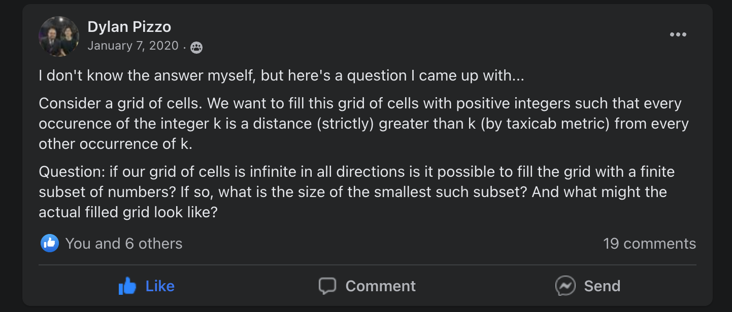
Now let us consider a more interesting example. Let \(\mathbb{Z}^2_\infty\) be the graph whose vertex set is \(\mathbb{Z}^2\), and that has edges not only between orthogonally adjacent vertices, but also diagonally adjacent pairs. Formally, for \(u, v \in \mathbb{Z}^2\), they are connected if \(\vert u - v \vert_\infty = 1\).

Now, if we consider the subgraph induced by any \((k+1) \times (k+1)\) subgrid of \(\mathbb{Z}^2_\infty\), we can only distance-color a single vertex \(v\) with color \(k\), as the other vertices of the subgraph are at distance at most \(k\) from \(v\). This means that color \(k\) has density at most \(\frac{1}{(k+1)^2}\). Therefore, even if we were to use colors \(1, \ldots, \infty\), the total fraction of the graph we could color would be at most:

This means \(\mathbb{Z}^2_\infty\) does not admit a distance-coloring with a finite number of colors. It even uses the cute Basel problem result for the infinite sum, how cool!

I discovered this that January, and of course the natural next step was to try to use the same strategy for the standard infinite grid \(\mathbb{Z}^2\) as the original Facebook post inquired. The problem is… this doesn’t work! If one considers a \((k+1) \times (k+1)\) subgrid of \(\mathbb{Z}^2\), it is possible to distance-color \(5\) different vertices with color \(k\) (1 in the center and 4 in the corners), so one ends up with a sum that is greater than \(1\), meaning it does not discard a finite coloring (note that if an infinite sum converges above 1, that means a finite prefix of it is enough to get past 1). So I started thinking that maybe for \(\mathbb{Z}^2\) there was a solution with finite colors. The problem was… I couldn’t find one!

To make things worse, I wasn’t making any interesting progress, so at some point I basically just let it go. Also, it’s worth mentioning that I tried googling about it, to see whether it had been solved before. At that point I would have been perfectly happy with finding a full solution online and calling it a day. But satisfying my mathematical curiosity on this one turned out to be much harder than that…

Also, some pretty important global events happened soon after the January 2020 summer school…

Flash-forward to September 2021. I enroll as a PhD student at Carnegie Mellon University. My main idea was to work on algorithms and discrete math with Anupam Gupta, whom I had met before in the Chilean Summer School of Discrete Mathematics. Now comes a pivotal point in this story. At CMU, one’s first semester as a Computer Science PhD student starts with an Introductory Course (IC) in which the different faculty present their research, and one is introduced to different aspects of life at CMU and in Pittsburgh.

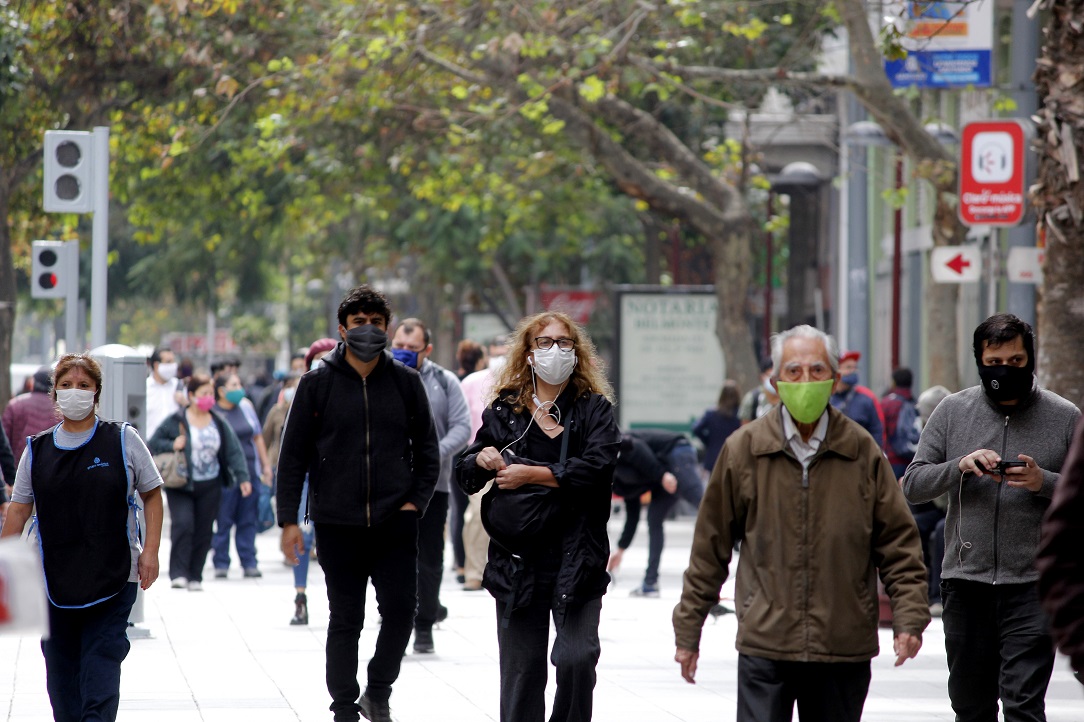
Marijn Heule gave his IC talk on his automated approach to the Pythagorean triples problem, which consists of coloring the integers with red and blue in a way that no Pythagorean triple is monochromatic. For example, if 12 and 16 receive color blue, then 20 must receive color red, as \(12^2 + 16^2 = 20^2\). It was a great talk, but also a 10-15 minutes one, directed to students with very different backgrounds and interests, so he couldn’t say anything very deep or technical. The main thing I got out of the talk was: “This CMU professor has been applying automated reasoning techniques to solve hard coloring problems; interesting.”

I didn’t know anything about automated reasoning techniques. So I e-mailed Marijn asking if we could chat for a little bit because I was wondering if “his automated reasoning techniques” could be applied to my silly Facebook-post coloring problem.

Marijn agreed to chat, and he liked the problem. Moreover, he was willing to work with me on it! This is actually quite rare in academia based on my personal experience. Professors love motivated students, but it’s generally risky for them to dive into a problem that occurred to the student; professors are usually pushing lines of research for the medium-long term, and usually have a way better grasp than students about which problems are solvable, and how impactful it would be to solve them. So it’s usually sub-optimal to sink their teeth into any random problem a student proposes. But Marijn was so intrigued by the problem that he was willing to guide me on it; to see if his techniques could be helpful for it, which he intuited to be the case.

Soon after, I was having lunch with Isaac Grosof, a 5th year PhD student at the time. Isaac is a truly brilliant student, one of those that shine blindingly bright even within a context as selective as a CMU CS PhD. I told them about the problem, and they liked it too. So much so that after we finished our lunch we went straight to their office and started to work on it together. We made a couple of simple observations I had already made on my own before, so I wasn’t terribly excited, and then Isaac had to leave for a meeting. If my recollection is right, I received an e-mail from them the next day, or at most 2 days later, with a partial solution to the problem. Isaac had found a way to color the infinite grid by using 23 colors in a periodic manner. To the best of my knowledge, they found this solution “manually” (i.e., trying things by hand on a computer, inspired by density arguments). I was completely blown away; it had only take Isaac a few hours to do something I had tried several times during the course of more than a year!

Marijn and I met shortly thereafter, and he explained me how to run a SAT solver on the problem. Armed with that, we were able to obtain a solution with 17 colors pretty quickly, and later that same week another solution with only 15 colors. Before understanding how a computer can be used to prove that 15 colors are enough to distance-color the infinite grid, it’s convenient to understand first how a computer can be used to prove that 3 colors are enough to distance-color the infinite path (which we know it’s possible from Figure 3). In order to do this, we can consider a subgraph of the infinite path, like \(P_4\), the path on 4 vertices, and try to distance-color it with \(3\) colors. Consider the following attempt¹:

The problem with the distance-coloring in Figure 9 is that we cannot extend it to the infinite path. The next vertex to the right must receive color \(1\), and the following one will not be able to receive any color. This is illustrated in Figure 10.

The question is therefore: how can find a distance-coloring of a finite path that can be extended to the infinite path, and hopefully in a periodic manner? The answer is: toroidal edges. The idea is that by connecting the endpoints of a finite path, and transforming it into a cycle, we will capture the property of the distance-coloring being periodically extendable; from a distance-coloring of \(C_4\) we can obtain a distance-coloring of \(C_8\), and thus for \(C_{16}\), and so on. This is illustrated next in Figure 11.

For showing that \(15\) colors are enough for a distance-coloring of the infinite grid we can proceed in a similar manner, by considering a \(72 \times 72\) subgrid of \(\mathbb{Z}^2\) with toroidal edges, meaning that the vertices of the left-most column of the subgrid are connected to the right-most column, and similarly top and bottom rows are connected.

The recipe for establishing coloring bounds on an infinite graph is thus as follows:

1. For establishing an upper bound (meaning that \(k\) colors are enough for the infinite graph), we need a finite subgraph with toroidal edges (i.e., edges that capture periodicity, in a way that guarantees that the coloring for the finite subgraph would allows us to obtain one for the infinite graph).²

2. For establishing a lower bound (meaning that \(k\) colors are not enough for the infinite graph), we simply need to show a finite subgraph for which \(k\) colors are not enough; if you can’t even color this finite tiny portion of the infinite graph, then no hope for the infinite graph!³

Both for finding a coloring of a finite subgraph, or showing that no coloring can exist with the target number of colors, we can use a SAT solver. The most direct SAT encoding for this problem is quite straightforward: if you have a graph \(G = (V, E)\), and want to decide whether it admits a distance-coloring with \(k\) colors, then create variables \(x_{v, c}\) representing that vertex \(v \in V\) gets color \(c \in \lbrace 1, \ldots, k \rbrace\), and add the following constraints:

1. Each vertex must get a color:

1. Vertices at distance at most \(c\) cannot share color \(c\):

Using this direct encoding over a \(72 \times 72\) subgrid with toroidal edges, and passing the resulting instance to a local search SAT solver, we obtained the following periodic solution:

Wow, we were making great progress! It was not hard to see that 9 colors were not enough, using some density arguments, but could 10 be enough? Maybe 11?

Marijn quickly came up with a very nice recursive SAT encoding for the problem, and after struggling to implement it (even though the idea is nice and simple, the details were quite tricky), we unfortunately discovered that it didn’t yield any practical improvements. It was asymptotically better, but in practice it turned out to be worse than the most direct and naive encoding. A constant of \(32\) can oftentimes be worse than a \(\log n\) factor!

I started to investigate related sub-problems, like the complexity of distance-colorings or the minimum number of colors required for other infinite graphs. I started to get some really cool results myself, which made me quite happy. Marijn was excited too.

A couple of months later we knew that 15 colors were enough and that one needed at least 13, that’s pretty close to a final answer!

But the terminology was bothering me. I was calling these “distance-colorings”, but I knew (as a quick Google search revealed), that people were using “distance-colorings” to refer to something else, and therefore I wanted a new term. I started doing an actual proper literary review (i.e., beyond a Google search) by reading surveys on different coloring problems, to see what was the nearest neighbor of our problem and figure out a related name. At some point during this literature review I stumbled upon this:

Despite the notation being different, this is actually the same problem! Wow, people knew about this! So I googled “packing chromatic number” and a survey came up. To my absolute horror (see Figure 14), a bunch of the results I had proved were already known, spread out over a dozen of papers (the survey cited over 60 papers on the topic!). Moreover, the survey mentioned that the packing chromatic number of the infinite square grid was… OPEN! and known to be between 13 and 15… The idea of packing colorings, and the problem of the infinite square grid had been posed 20 years ago, in 2002! As a fun fact, the first upper bound, obtained by Goddard et al. in their seminal paper introducing these colorings, was 23, the same number Isaac Grosof had obtained manually!

I was horrified. I had basically been working for several months on a problem without realizing this, and even worse, I had made Marijn waste his time on it! So I e-mailed him asking for a quick meeting ASAP, which I was extremely nervous about. But Marijn’s reaction was incredible: he was actually happy instead of upset! He was happy that other people cared about the problem, and he was happy that the original core part of the problem, that of determining the packing-chromatic number of the infinite square grid, was still open. Needless to say, I was very relieved.

So Marijn and I started pushing to improve the \(13 \leq \chi_\rho(\mathbb{Z}^2) \leq 15\) gap (note that our notation has changed from \(\chi_d(\cdot)\) to \(\chi_\rho(\cdot)\)!), and in a few months, after several optimizations and discussions and dozens of experiments, we managed to prove the answer was not 13. At this point the title of the paper we wrote about it is not hard to guess: “The Packing Chromatic Number of the Infinite Square Grid is At Least 14”. It got accepted at SAT’2022 🙂.

One of the simplest optimizations we used, for example, is symmetry breaking. The idea of symmetry breaking is that CDCL SAT solvers can be understood as programs that try the different Boolean assignments in a way that’s more clever than simply iterating over the \(2^{\# {\rm vars}}\) possibilities, and they do this by learning things from the partial assignments they try. As the following figure shows, many of these partial assignments can be symmetric, which means that exploring them separately is a waste of time.

A way to avoid this waste of time is by breaking the symmetry, meaning that by incorporating additional restrictions the instance is no longer symmetric. In the case of a diamond subgraph, we can add the following constraint: “the occurrence of the largest color that appears the closest to the center must appear in the north-north-east octant”, thus gaining a factor of 8 in runtime.

After even more rounds of experiments, optimizations and meetings, we had proved that the answer was at least 14, and it had taken all the optimizations and ideas we had. To prove that the answer was actually 15, meaning that 14 colors were not enough, we pretty much needed to optimize our computation by a factor of roughly 100. Note that a really nice optimization idea sometimes gives you a factor of 2, so you’d need 7 of those ideas to improve by a factor of 100!

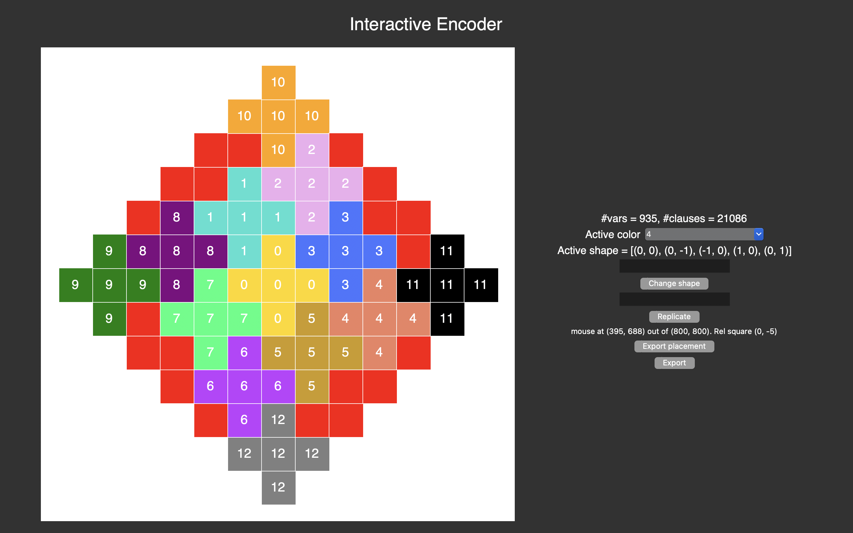
But Marijn had faith in us solving the problem, so we kept working on it. We started reverse engineering automatic tools to see how they operated in this particular problem, and we started learning from that. At this point I was playing around with 20 different ideas a week; I had made some visual interactive interfaces where I could try out optimization ideas more quickly by clicking on stuff with my mouse instead of writing code for each optimization.

We were getting closer and closer to the result, but we were still missing more optimizations. Let me present in the next paragraph one of the coolest results from this project:

When trying to find packing-colorings for the infinite grid, and also for the \(D_r\) graphs (i.e., diamond of radius \(r\)), color \(1\) is the most helpful, as it can have a density of \(\frac{1}{2}\) (i.e., cover half of the graph). For example, in Figure 12, out of the \(72 \times 72 = 5184\) vertices, exactly \(2592 = \frac{5184}{2}\) receive color \(1\). At this point, we were conjecturing that using color \(1\) in the chessboard pattern that yields density \(\frac{1}{2}\) was optimal, meaning that you could packing-color a graph \(D_r\) with \(k\) colors (forcing any color \(c \neq 1\) in the center, this is called a \(D_{r, k, c}\) instance) if, and only if, you could do it enforcing the chessboard pattern of \(1\)’s. The motivation to prove this conjecture was very simple: if true, then by enforcing the chessboard pattern of \(1\)’s the number of vertices would go effectively down by half (as the vertices colored \(1\) don’t need to be included in the encoding). Note that in a problem whose runtime is exponential on the input size, reducing the input size by a factor of 2 is monumental; runtime goes down to its square root!

In fact, we quickly managed to prove that assuming the chessboard conjecture was true, then that would imply \(\chi_\rho(\mathbb{Z}^2) = 15\), the answer we suspected. So I was trying really hard to prove this conjecture by pen and paper, but was failing equally hard at the task…

After more optimizations, it turned out the chessboard conjecture was false, and our optimized techniques allowed us to find the smallest counterexample!

But this didn’t stop us, we kept optimizing and after a couple more months we finally managed to solve the problem. We had proved that 14 colors weren’t enough! Really exciting! \(\chi_\rho(\mathbb{Z}^2) = 15\)! This was roughly 3 years after I first discovered the problem. A summary of the historical progress on the problem is presented below:

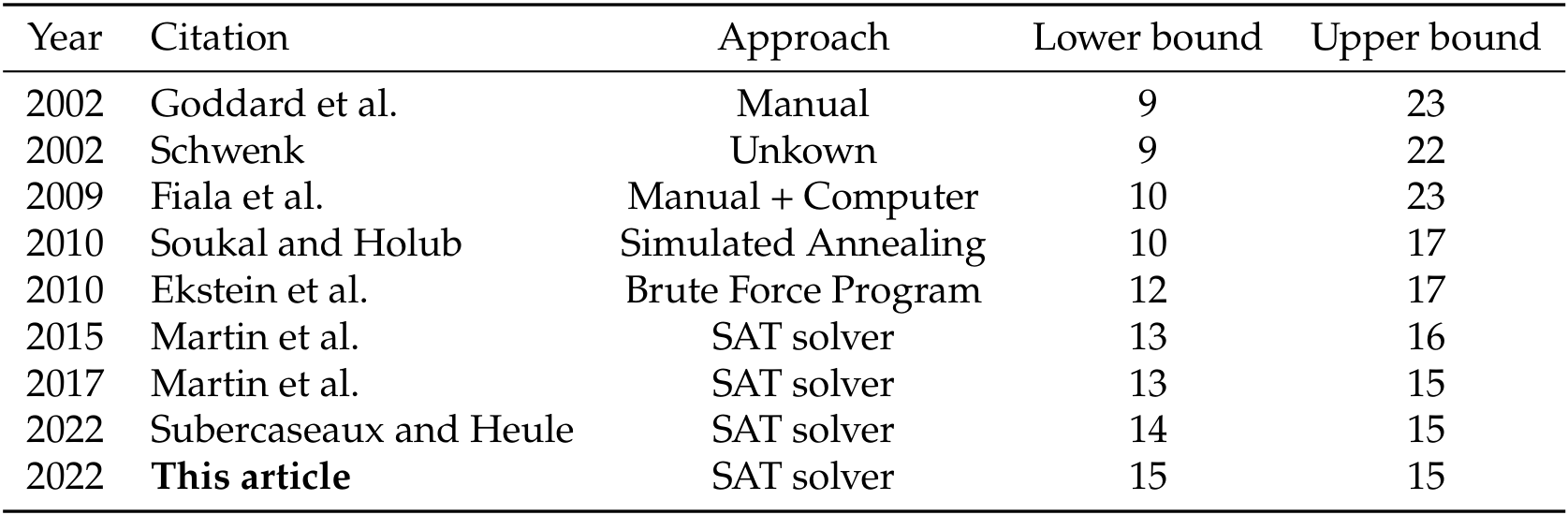
For a point of reference on much we optimized, in 2010, Ekstein et al. proved a lower bound of 12, and it took them 120 days of computation, whereas our techniques allow us to get the same lower bound in less than 10 seconds. This is a x1000000 factor improvement! Admittedly, hardware has improved substantially since 2010, but we went far beyond the hardware speed-up.

There was however one crucial part missing: how could we be sure that all our code and all our optimizations and all our symmetry breaking was correct? Marijn and I started working on generating a single automated proof, which could be then checked by an independent verified checker. This turned out to be a tricky endeavor, and moreover, we found several mistakes in our code during the process! Fortunately, all the bugs we found were fixable, and thus we ended up with a fully verified proof. To be a bit more precise, the exact theorem we proved is: assuming the direct encoding shown above is correct, then \(\chi_\rho(\mathbb{Z}^2) = 15.\) This means the only unverified part is the correctness of the direct encoding (which corresponds to only 26 lines of Python).

The solution to the problem took a total of 4851 CPU hours (we used a supercomputer with 128 cores!), and verifying the proof took another 4336 CPU hours. The total uncompressed proof weighed 122 terabytes! and only 34 terabytes after compression.

Finally, we wrote a paper for TACAS’2023 with this final result. The title is not hard to guess: “The Packing Chromatic Number of the Infinite Square Grid is 15”. We have put up an arXiv version!

Donald Knuth, one of my all-time Computer Science heros, happens to know my advisor Marijn, so he read a draft of our TACAS paper. Knuth, my idol, was reading a paper I co-authored! He gave us extremely careful feedback and suggestions: there was not a single typo he missed! In fact, the reviews we got from the conference were almost a subset of Knuth’s extensive feedback. At the end of his long email he wrote a high-level review:

In general, of course, I found this paper extremely interesting and stimulating. The ideas are presented lucidly and in a well motivated way; the illustrations are wonderful. I agree with the remark on page 16 that “split-encoding compatibility” is probably the innovation most likely to become widely applicable to other problems. (I love “reverse engineering” of mechanical optimizations! That’s how I once came up with my 1/3 of the “Knuth-Morris-Pratt” algorithm, for instance: Steve Cook had published a mechanical way to convert small-space stack automata into small-time random-access-machine code.)

Best regards, Don

Also, Knuth wrote us that he believes the chessboard conjecture might still be true for diamonds of odd radius! I couldn’t be happier! This little problem, taken from a Facebook group, has given me so much joy! Some frustration at times, but mostly joy. The paper of Martin et al. from 2017, in which they proved the answer to be between 13 and 15, contains the following quote:

“The first author heard of this problem at a talk by Bernard Lidicky at the 8th Slovenian Conference on Graph Theory (Bled 2011). While this problem may not be especially important, few who worked on it can doubt that it is very addictive, and further provides a vehicle through which to ponder different algorithmic techniques. One of the curiosities of the problem is that we have little theoretical insight into it.”

This problem was definitely very addictive to me too!

To close this post, I’ll circle back all the way to Coq, the theorem prover. During the Coq summer school I learned about the importance of verified proofs, which ended up having significant research implications for me years later! I’ve now started using Lean (another theorem prover) to verify my proofs on some unrelated mathematical problems. Furthermore, Yong Kiam Tan, a CMU alumni who has worked with Marijn, verified our direct encoding in CakeML (yet another theorem prover), meaning that now every single bit of our proof has been verified!