Suppose we have a collection of binary vectors that we wish to store. If many of them are similar, storing each vector independently would be wasteful. Instead, we can use delta compression: store one vector explicitly, and represent each of the others by a pointer to another vector, together with the positions at which they differ. (Imagine the memory savings at Github by storing only the code diffs as opposed to each full version!)

For example, consider these six vectors:

x₁ = 1 0 0 1 0 1
x₂ = 1 0 1 0 0 1
x₃ = 1 0 0 1 1 1
x₄ = 1 0 1 1 0 1
x₅ = 1 1 0 1 0 1
x₆ = 1 0 1 0 0 0

We could store \(x_1\) explicitly, and then store \(x_2\) by saying “take \(x_1\) and flip positions 3 and 4.” We could then describe \(x_3\) relative to \(x_2\), and so on. But the order matters! Describing each vector relative to the preceding one requires a total of 13 coordinate changes. If we choose the parents more carefully, we only need 5.

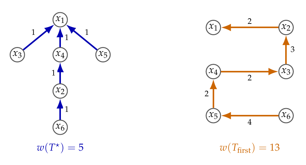
Naturally, for vectors with only six coordinates, storing pointers and lists of indices is not actually a compression improvement. The point of the example is the choice of parents. For large, repetitive data, this choice can make a substantial difference.

More precisely, given \(n\) vectors in \(\{0,1\}^d\), consider the complete graph whose edge weights are their Hamming distances, i.e., the number of coordinates at which they differ. A minimum spanning tree (MST) minimizes the total number of coordinate changes in this tree-based representation.

The main obstacle, however, is computing that tree.

The distances are not a given!

Prim’s algorithm computes an MST in \(O(n^2)\) time on a complete graph. But this assumes constant-time access to the edge weights. Here, we are given vectors, not distances, and comparing two vectors takes \(\Theta(\lceil d/w\rceil)\) word operations, where \(w\) is the machine word size. Computing all pairwise distances first therefore costs \(\Theta(n^2\lceil d/w\rceil)\).

The goal of this note is to remove the dimension factor from the quadratic term, at the cost of an arbitrarily small multiplicative error. For any fixed \(\varepsilon>0\), we can compute a tree whose weight is at most \(1+\varepsilon\) times the optimum in \(O(n^2+nd)\) time, with high probability.

The more precise bound is \(O(\varepsilon^{-3}(n^2+nd))\), on a word-RAM with word size \(\Theta(\log(nd))\), for \(1/(nd)\leq\varepsilon\leq1\). This is still quadratic in the number of vectors; the improvement is that we no longer multiply that quadratic term by their dimension.

In my case, the motivation came from the recent work of Cardinal, McCarty, and Yuditsky. Roughly speaking, they showed that if the neighborhoods of a graph admit a succinct delta representation, then the graph also admits a succinct biclique partition: a representation of its edges as a disjoint union of complete bipartite graphs. Their result improved upon previous work I participated in, but more importantly, it provides an algorithmic path toward constructing compact biclique representations of structured graphs. These can in turn be used to construct efficient SAT encodings, as discussed in my earlier post.

The bottleneck in their construction was an approximate MST in Hamming space. Improving that step lets us construct a biclique partition of the same quality in \(O(n^2)\) time instead of \(O(n^2\log n)\).

Local to global approximations

Let us first make a simple observation. Prim grows a tree on a set \(S\) by repeatedly choosing a lightest edge from \(S\) to a vertex outside it. Suppose that, instead, we always choose an edge that is at most \(\alpha\) times heavier than the lightest edge across that cut. Then the final tree is an \(\alpha\)-approximation of the MST. That is, a local \(\alpha\)-approximation translates into a global one.

The proof is a short exchange argument (which I got from my friend Arturo Merino). Start with an optimal MST, with all its edges colored red. Whenever our approximate Prim chooses an edge, we color it blue. The invariant is that, all blue edges lie inside the current set \(S\). Now, whenever the edge chosen by approximate Prim wasn’t colored before, it becomes part of a colored cycle, and hence we can remove a red edge crossing the same cut (we know the other edge crossing the cut is red by our invariant). The new edge costs at most \(\alpha\) times the red edge it replaces. If the chosen edge was already present, simply recolor it. At the end, every original edge has been replaced or recolored exactly once, increasing its cost by a factor at most \(\alpha\), so summing these inequalities gives the desired guarantee.

A small sketch for a distance question

The distance tool comes from the parity sketches of Kushilevitz, Ostrovsky, and Rabani. Fix a distance scale \(R>1\). Select each coordinate independently with probability \(1/(2R)\), using the same selected coordinates for every vector. Record, for each vector, the parity of its selected bits. This gives a one-bit sketch.

Now suppose that two vectors differ in exactly \(m\) coordinates. Their sketch bits differ precisely when an odd number of those coordinates were selected. A standard parity calculation gives

To get some intuition, the right-hand side is approximately \(\frac12(1-e^{-m/R})\). When \(m\ll R\), it is close to zero, whereas for \(m\gg R\) it approaches \(1/2\). Repeating this experiment gives us a pretty good idea of whether the distance is below or above the scale we care about.

Of course, distinguishing distances extremely close to \(R\) requires more care. We use scales \(\rho^j\), where \(\rho=1+\varepsilon/4\), and allow a small gap: a test at scale \(j\) accepts distances at most \(\rho^{j-1}\) and rejects distances at least \(\rho^j\). Inside that gap the test makes no promise.

Choosing \(L:=O(\varepsilon^{-1}\log(2d))\) scales, and \(O(\varepsilon^{-2}\log(nL))\) repetitions per scale makes all tests reliable simultaneously, with high probability. Packing those bits into machine words makes one test cost \(O(\varepsilon^{-2})\) word operations, rather than a scan through the original vectors.

Only ask whether the new parent is sizably better

We could now approximate every pairwise distance, but that would be doing more work than Prim needs. For each vertex \(u\) outside the current tree, we keep a candidate parent \(p(u)\in S\) and a level \(\ell(u)\). The value \(\rho^{\ell(u)}\) is an upper estimate for the distance to its parent.

When a new vertex \(b\) enters the tree, we ask whether it would improve the current estimate for \(u\) by a whole scale. If the test at scale \(\ell(u)-1\) accepts, we make \(b\) the new parent, decrease \(\ell(u)\), and try again. We stop at the first failed test, or when the level reaches 1. To grow the tree, we choose an outside vertex with minimum level and add its parent edge.

Why is this enough? After processing the current tree, we maintain two facts:

Here \(\Delta\) denotes Hamming distance. The first inequality says that the parent really witnesses our upper estimate. The second says that no vertex already in the tree is substantially closer. A failed test gives the second inequality for the newly inserted vertex, and lowering a level only makes it easier to satisfy for the old ones. At level 1, the lower bound follows because distinct vectors have distance at least 1. Duplicate vectors can be removed at the start and reattached by zero-weight edges at the end.

The two estimates differ by only a factor \(\rho^2\leq1+\varepsilon\). Choosing a minimum-level vertex therefore gives an edge within that factor of the lightest edge across the cut. Our approximate-Prim observation does the rest.

The nice part is the running-time accounting. We can have one failed test for each pair of vertices, giving \(O(n^2)\) failures. Every successful test decreases a level, and levels never go back up. Across the entire algorithm, there can therefore be only \(O(nL)\) successes.

There is still some work hidden in constructing the sketches, since doing it naively could ruin our bound, but that part is essentially a technical annoyance.

So the ingredients are quite classical: Prim, parity sketches, and a short amortized analysis. The useful observation is that we do not need to learn each distance accurately; we only need to know whether a new parent is substantially better.